demo23_focal.py

"""演示23: 类别不平衡 — 交叉熵 vs Focal Loss。

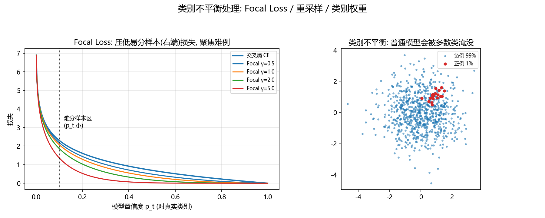
在极不平衡二分类(正例占 1%)上比较普通交叉熵与 Focal Loss 的损失曲线与
"易分样本抑制"效果。Focal Loss: FL = -(1-p_t)^γ · log(p_t)。
"""
import os
import numpy as np
import matplotlib.pyplot as plt
from figure_style import figures_dir, configure

configure()

OUT = figures_dir()
os.makedirs(OUT, exist_ok=True)


def ce(p):
    return -np.log(np.clip(p, 1e-6, 1))


def focal(p, gamma=2.0):
    return -(1 - p) ** gamma * np.log(np.clip(p, 1e-6, 1))


p = np.linspace(0.001, 0.999, 500)
fig, (ax1, ax2) = plt.subplots(1, 2, figsize=(12, 4.8))

# ① 损失曲线
ax1.plot(p, ce(p), "tab:blue", lw=2, label="交叉熵 CE")
for g in (0.5, 1.0, 2.0, 5.0):
    ax1.plot(p, focal(p, g), lw=1.6, label=f"Focal γ={g}")
ax1.axvline(0.1, color="k", ls=":", lw=0.8)
ax1.text(0.12, 3.0, "难分样本区\n(p_t 小)", fontsize=9)
ax1.set_xlabel("模型置信度 p_t (对真实类别)"); ax1.set_ylabel("损失")
ax1.set_title("Focal Loss: 压低易分样本(右端)损失, 聚焦难例")
ax1.legend(fontsize=8); ax1.grid(alpha=0.3)

# ② 类别不平衡示意
fig2 = ax2
rng = np.random.default_rng(0)
pos = rng.normal([1, 1], 0.4, (20, 2))
neg = rng.normal([0, 0], 1.2, (800, 2))
ax2.scatter(neg[:, 0], neg[:, 1], c="tab:blue", s=5, alpha=0.5, label="负例 99%")
ax2.scatter(pos[:, 0], pos[:, 1], c="tab:red", s=15, label="正例 1%")
ax2.set_title("类别不平衡: 普通模型会被多数类淹没")
ax2.legend(fontsize=8); ax2.set_aspect("equal")

fig.suptitle("类别不平衡处理: Focal Loss / 重采样 / 类别权重", fontsize=14)
fig.tight_layout(rect=(0, 0, 1, 0.93))
out = os.path.join(OUT, "fig_train_imbalance.png")
fig.savefig(out, dpi=150)
print(f"-> {out}")