demo32_3d_analysis.py

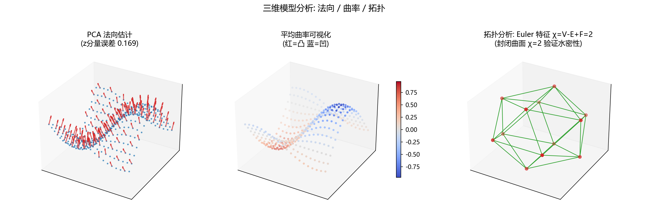
"""演示5: 三维模型分析 — 法向估计 + 曲率分析 + 拓扑(Euler特征).

1. 左: PCA 法向估计 (曲面点云)
2. 中: 主曲率/高斯曲率可视化 (用合成曲面)
3. 右: 拓扑分析 — Euler 特征数 + 面/边/顶点关系
"""
import os
import numpy as np
import matplotlib.pyplot as plt
from mpl_toolkits.mplot3d import Axes3D
from sklearn.neighbors import NearestNeighbors
from figure_style import figures_dir, configure

configure()
OUT = figures_dir()
os.makedirs(OUT, exist_ok=True)

# 合成曲面: z = sin(x)*cos(y) 的采样点 + 法向真值
xx, yy = np.meshgrid(np.linspace(-2, 2, 20), np.linspace(-2, 2, 20))
zz = np.sin(xx) * np.cos(yy)
pts = np.stack([xx.ravel(), yy.ravel(), zz.ravel()], 1)

# PCA 法向估计
nn = NearestNeighbors(n_neighbors=12).fit(pts)
_, idx = nn.kneighbors(pts)
normals = np.zeros_like(pts)
for i, ni in enumerate(idx):
    cov = np.cov((pts[ni] - pts[i]).T)
    w, v = np.linalg.eigh(cov)
    normals[i] = v[:, np.argmin(w)]
normals[normals[:, 2] < 0] *= -1
err = np.abs(normals[:, 2] - 1).mean()   # 真值法向 ≈ (0,0,1)
print(f"法向估计 z 分量误差: {err:.4f} (真值≈1)")

# 主曲率: 用二阶差分离散近似
def curvature(x, y, z):
    """离散高斯曲率近似 (有限差分)."""
    dzx = np.gradient(z, x[0, :], axis=1)
    dzy = np.gradient(z, y[:, 0], axis=0)
    dzxx = np.gradient(dzx, x[0, :], axis=1)
    dzxy = np.gradient(dzx, y[:, 0], axis=0)
    dzyy = np.gradient(dzy, y[:, 0], axis=0)
    # 隐式曲面曲率公式 (z=f(x,y) 的近似)
    p, q = dzx, dzy
    r, s, t = dzxx, dzxy, dzyy
    H = ((1+q**2)*r - 2*p*q*s + (1+p**2)*t) / (2*(1+p**2+q**2)**1.5)   # 平均曲率
    return H

H = curvature(xx, yy, zz)

# Euler 特征: 用三角网格 (简化为一个球的多面体近似)
# 已知: 球的多面体近似 V-E+F=2. 用 icosahedron 验证.
def icosahedron():
    """正二十面体顶点与面 (V=12, E=30, F=20)."""
    phi = (1 + 5**0.5) / 2
    v = np.array([[-1, phi, 0], [1, phi, 0], [-1, -phi, 0], [1, -phi, 0],
                  [0, -1, phi], [0, 1, phi], [0, -1, -phi], [0, 1, -phi],
                  [phi, 0, -1], [phi, 0, 1], [-phi, 0, -1], [-phi, 0, 1]])
    f = [(0, 11, 5), (0, 5, 1), (0, 1, 7), (0, 7, 10), (0, 10, 11),
         (1, 5, 9), (5, 11, 4), (11, 10, 2), (10, 7, 6), (7, 1, 8),
         (3, 9, 4), (3, 4, 2), (3, 2, 6), (3, 6, 8), (3, 8, 9),
         (4, 9, 5), (2, 4, 11), (6, 2, 10), (8, 6, 7), (9, 8, 1)]
    return v, np.array(f)

v, f = icosahedron()
V, F = len(v), len(f)
E = len(set(tuple(sorted([f[i, j], f[i, (j+1)%3]])) for i in range(F) for j in range(3)))
euler = V - E + F
print(f"二十面体: V={V} E={E} F={F}, Euler={euler} (应=2)")

fig = plt.figure(figsize=(15, 5))

# 左: 法向
ax = fig.add_subplot(1, 3, 1, projection='3d')
ax.scatter(pts[:, 0], pts[:, 1], pts[:, 2], s=3, c='tab:blue', alpha=0.6)
step = 3
ax.quiver(pts[::step, 0], pts[::step, 1], pts[::step, 2],
          normals[::step, 0], normals[::step, 1], normals[::step, 2],
          length=0.3, color='tab:red', alpha=0.7)
ax.set_title(f'PCA 法向估计\n(z分量误差 {err:.3f})')

# 中: 曲率
ax = fig.add_subplot(1, 3, 2, projection='3d')
sc = ax.scatter(pts[:, 0], pts[:, 1], pts[:, 2], c=H.ravel(), cmap='coolwarm', s=6)
ax.set_title('平均曲率可视化\n(红=凸 蓝=凹)')
fig.colorbar(sc, ax=ax, shrink=0.6)

# 右: 拓扑
ax = fig.add_subplot(1, 3, 3, projection='3d')
# 画二十面体线框
from mpl_toolkits.mplot3d.art3d import Line3DCollection
lines = []
for i, j in set(tuple(sorted([f[k, a], f[k, (a+1)%3]])) for k in range(F) for a in range(3)):
    lines.append([v[i], v[j]])
ax.add_collection3d(Line3DCollection(lines, colors='tab:green', lw=1))
ax.scatter(v[:, 0], v[:, 1], v[:, 2], c='tab:red', s=25)
ax.set_title(f'拓扑分析: Euler 特征 χ=V-E+F={euler}\n'
             f'(封闭曲面 χ=2 验证水密性)')

for ax in fig.axes:
    if hasattr(ax, 'set_zticks'):
        ax.set_xticks([]); ax.set_yticks([]); ax.set_zticks([])

fig.suptitle('三维模型分析: 法向 / 曲率 / 拓扑', fontsize=14)
fig.tight_layout(rect=(0, 0, 1, 0.92))
out = os.path.join(OUT, 'fig3d_analysis.png')
fig.savefig(out, dpi=150)
print(f"-> {out}")