12345678910111213141516171819202122232425262728293031323334353637383940414243444546474849505152535455565758596061626364656667686970717273747576 |
"""演示19: 激活函数与损失函数 — 非线性来源与训练目标。

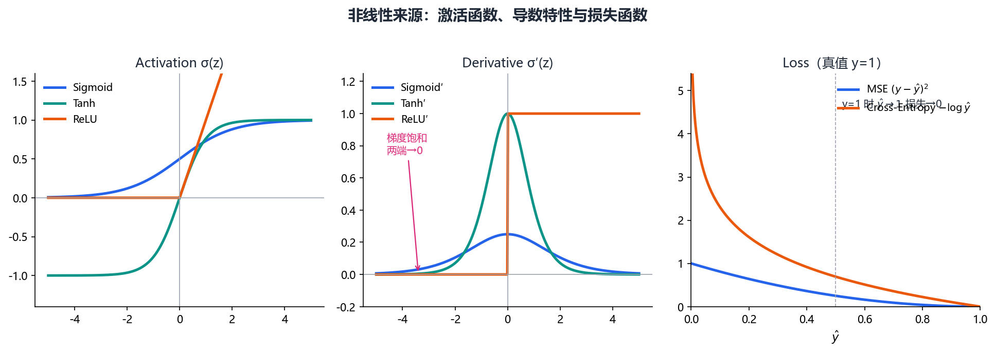
1. 激活函数: Sigmoid / ReLU / Tanh 曲线及其导数(梯度饱和现象直观可见)。
2. 损失函数: MSE 与 交叉熵 在二分类上的形状对比。
"""
import os
import numpy as np
import matplotlib.pyplot as plt
from figure_style import figures_dir, configure

configure()

OUT = figures_dir()
os.makedirs(OUT, exist_ok=True)

z = np.linspace(-6, 6, 400)


def sigmoid(z):
    return 1 / (1 + np.exp(-z))


def d_sigmoid(z):
    s = sigmoid(z)
    return s * (1 - s)          # 两端饱和 -> 梯度趋近 0


def relu(z):
    return np.maximum(0, z)


def d_relu(z):
    return (z > 0).astype(float)   # 负区间导数为 0 -> "死亡 ReLU"


def tanh(z):
    return np.tanh(z)


def d_tanh(z):
    return 1 - np.tanh(z) ** 2

fig, axes = plt.subplots(1, 2, figsize=(12, 4.8))

# ① 激活函数 + 导数
ax = axes[0]
for name, fn, dfn, color in [
        ("Sigmoid", sigmoid, d_sigmoid, "tab:blue"),
        ("ReLU", relu, d_relu, "tab:green"),
        ("Tanh", tanh, d_tanh, "tab:orange")]:
    ax.plot(z, fn(z), color, lw=2, label=f"{name}")
    ax.plot(z, dfn(z), color, lw=1.2, ls="--", alpha=0.6, label=f"{name} 导数")
ax.axhline(0, color="k", lw=0.6)
ax.set_title("激活函数 (实线) 及其导数 (虚线): 引入非线性")
ax.legend(fontsize=8); ax.grid(alpha=0.3)

# ② 损失函数: 二分类, 真实标签 y=1
ax = axes[1]
y_true = 1.0
p = np.linspace(1e-3, 1 - 1e-3, 400)          # 预测概率
mse = (y_true - p) ** 2
ce = -(y_true * np.log(p) + (1 - y_true) * np.log(1 - p))
ax.plot(p, mse, "tab:blue", lw=2, label="MSE (回归)")
ax.plot(p, ce, "tab:red", lw=2, label="交叉熵 (分类)")
ax.axvline(y_true, color="k", ls=":", lw=0.8)
ax.set_xlabel("预测概率 p"); ax.set_ylabel("损失 L")
ax.set_title("损失函数: 预测与真实的差距度量")
ax.legend(); ax.grid(alpha=0.3)
ax.set_xlim(0, 1)

fig.suptitle("感知机/全连接的「非线性来源」与「训练目标」", fontsize=14)
fig.tight_layout(rect=(0, 0, 1, 0.93))
out = os.path.join(OUT, "fig_ai_activation_loss.png")
fig.savefig(out, dpi=150)
print(f"-> {out}")
|